Marquee

Do you need a website for your Church, School, Business or NGO? Just give us a call: +233 24 311 5791 or +233 20 909 1616

Monday 28 August 2017

Using "PMT" Function to Calculate for Loan Payments in Excel


The Excel PMT function calculates the repayment amount for a loan or the constant periodic payment required to pay off a loan, with a constant interest rate, over a specific year or period

The syntax PMT is: =PMT(rate,nper,pv)

Where the arguments are as follows:
  • rate:     The interest rate, per period
  • nper:    The number of years or periods over which the loan is to be paid
  • pv:        The present value of the loan or investment

Cash Flow Convention:

Note: In line with the general cash flow convention, outgoing payments are represented by negative numbers and incoming payments are represented by positive numbers

In this exercise, we will practice by learning how to calculate the monthly payments on loans by some individuals which are to be paid off in full after some period of years.  Interest is charged at a rate of 5% and the payment to the loans are to be made at the end of every month.
  • Open to MS Excel and enter the following fictitious data into the spreadsheet:
  • Save the workbook as Loan Payment in a private folder or on a Flash drive
    Optional: Download our Practice Workbook

Step 1:           Converting the Loan Amount into an Accounting format

We will now convert the “Loan Amount values into a currency format of your preference.  In our example, we will use GHC currency format.  To do this, execute the following steps:
  • Highlight the cell range B4:B13
  • On the Home tab, click on Number Format dialog box launcher
The Format Cells dialog box appears
  • In the Category area, click on Currency or Accounting
  • In the Sample area, click on Symbol drop down list, scroll down and select GHC

Note:  You can press GH on the keyboard to quickly select GHC currency from the list
  • When done, click on [OK] button
Result:

Step 2:           Calculating for the RATE

This is done by dividing the Interest by a year (i.e. 12 per month)

Note:  Cell C4 will be treated as absolute reference (i.e. $C4$4)

To do this, execute the following steps:
  • In cell E4, type:       =$C$4/12
  • Press the [Enter] key to complete the formula
The formula result is:          0.004167
  • AutoFill cell E4 through cell E13
This means each client will be charged 0.004167 as the Rate

Step 3:          Calculating for the NO. OF PAYMENTS (Nper)

This is done by multiplying the No. of Years by 12 months.  To do this, execute the following steps:
  • In cell F4, type:        =D4*12
  • Press the [Enter] key to complete the formula
The formula result is:          36

AutoFill cell F4 through cell F13

Result:

Step 4:      Calculating for the MONTHLY PAYMENT (Pmt)

This is done by dividing the “Rate by 12 month and then multiply the “No. of Years by 12 month per the “Loan Amount (Pv)

In this case, we will use the PMT function to calculate for the Monthly Payment.  To do this, execute the following steps:
  • Click in cell G4
  • On the Formulas tab, click on Financial and select PMT function
The PMT function dialog box will pop up
  • Enter the following data into their respective text boxes:
  • In ‘Rate’ text box, type:      $C$4/12
  • In ‘Nper’ text box, type:      D4*12
  • In ‘Pv’ text box, type:         B4
The PMT settings should be configured as the one shown below:

  • Click on [OK] button to complete the formula

The syntax of the PMT function reads:      =PMT($C$4/12,D4*12,B4)

The formula result is:          -£224.78

Formula Explanations:
Excel calculates the interest rate by dividing it by 12 months and then multiples the number of years over which the loan is to be paid by 12 months per the loan amount

As explained earlier, the formula for the PMT function is: =PMT(rate,nper,pv)

ü  rate   =       5%/year which equals 5/12 per month
ü  nper   =       36 years × 12 months
ü  pv      =       7,500.00 (This is what we barrowed from the bank)

Note: 
Excel returns a negative payment value of -£224.78.  This is because a payment is considered as an out-going, and therefore a negative value is returned. 

We need to convert this negative value to a positive value (because this is how we normally think of money).

To avoid negative payment as an answer, we need to edit our formula by placing a minus sign () before B4 in the formula; so it looks –B4. To do this, execute the following steps:


  • Activate cell G4
  • In the formula bar, click before B4 and type a minus sign [-]
The syntax of the PMT function now reads:          =PMT($C$4/12,D5*12,-B4)


  • Press the [Enter] to complete the formula
  • AutoFill cell G4 through cell G13
Result:

Step 5:           Calculating for the Total Pay Back

Total Pay Back is the total amount that will be paid to the bank.  This is done by multiplying the “No. of Payments (Nper) byMonthly Payment (Pmt)


  • In cell H4, type:       =F4*G4
  • Press the [Enter] key to complete the formula
The formula result is:          £8,092.14


  • AutoFill cell H4 through cell H13
  • Select the cell range G4:H13 and convert them into GHC currency format
Result:


Note:
When formatting cells, the resulting number may at times be quite large to fully display in the cell.  In this case, you may see ######## in the cells.  When this happens, expand the column width to display the values in the cells.

Final Result:


Overview:
The Total Pay Back of a loan over 10 years (i.e. GHC445,475.16) does not look so attractive. This means, the longer the duration of the loan, the more interest payment


Watch out for the next tutorial

Comments:
Kindly leave your comments, suggestions and critics on my Contact page because these will help improve the weblog and be of help to others.

Please, don’t forget to share with others.

Thank you.

Monday 7 August 2017

Using “Rank” Function pto Determine Position in MS Excel


The Rank function determines the relative position or order of one value in a range of data compared to the other values in the same range of data.

This means it is not necessary to sort data in either ascending or descending order to see the relative rankings of values in a data range.  For example: 1st, 5th, 3rd, 6th, 2nd, 4th, etc.

The RANK function has two (2) sections with a comma (,) between each section:

=RANK(number,ref)

In our tutorial, we will create a Quiz Scoreboard template using the Rank function to determine the contestant’s positions.

There are ten (10) schools with each answering four (4) rounds of questions in the quiz competition.

We assume you have a basic understanding of MS Excel cell references, autofill, finding the total, MAX, MIN, AVERAGE etc. and other basic operations.

Step 1             Entering data into the spreadsheet       

·         Enter the following fictitious data shown below exactly as they appeared into the spread sheet:


·         Save the worksheet as Quiz Scoreboard in a private folder or on a flash drive

Step 2             Finding the Total score      

We will configure the Total place holder for each school

·         Click in cell G2 and type:     =SUM(C2:F2)
·         Press the [Enter] key to complete the formula

The formula result is:          0

Since no data has been entered for any of the rounds, the Total score records zero (0)

Instead of calculating the Total for each school, we will let Excel do its magic by using the AutoFill command to copy the formula to other cells

Note:

AutoFill is a command used to extend series of formulas, numbers and/or texts to other cells.  The AutoFill handle is a tiny black-plus (+) sign which is displayed when the cursor is moved to the bottom-right corner of the active cell

To AutoFill, execute the following steps:


·         Click in cell G2 and locate the AutoFill handle at the bottom-right corner of the cell as shown below:

·         Double-click on the AutoFill handle to copy the formula

Result:

Step 2             Finding the Position           

We will configure the Position place holder for each school

In this case, we will use the “Rank function to configure the Position for each school based on their Total scores

·         Click in cell H2
·            On the Formulas tab, click on More Function, point to Compatibility, scroll down and select RANK


Note: This will display the Rank dialog box.  You can drag the dialog box to any place on your screen to enable you view the table

·         Enter the following information into their respective text boxes:
          ü   In the ‘Number’ text box, type:          G2
ü   In the ‘Ref’ text box, type:                G2:G11
·         Press [F4] function key to insert the dollar ($) sign (i.e. $G$4:$G$11)

Note:  The $ symbol in $G$4:$G$11 means Absolute Cell Reference.  Meaning Excel will treat the cell range G2:G11 as a unique range. (i.e. from OLA SHS to TANYIGBE SHS)

The Rank dialog box should look like this:


·         Click on [OK] button to complete the formula

The syntax for the formula in the Formula bar reads:     =Rank(G2,$G$2:$G$11)

The formula result is:          1

·         AutoFill cell H2 through cell H11


Since zero (0) is conceded as a number, excel assumed it to be a record for Total scores and thus displays one (1) for the Positions

We will now test our formula created for Total and Position respectively by entering marks for Round 1.

·         Enter the following fictitious data for Round 1 into the table:


Result:


From the quiz scoreboard, St. Paul’s SHS is in a comfortable lead, followed by Mawuli SHS.

We will now complete our Quiz scoreboard by entering the following fictitious data for Round 2, Round 3 and Round 4 respectively


Final Result:

In the final round, St. Mary’s Sem. SHS scored 32 points and thus came 1st position, Bishop Herman College scored 27 points and came second and the list goes on

Source: BB Series

Sunday 6 August 2017

Steps to Design an Elegant TV3 Logo


In this tutorial, you will learn how to use the pre-illustrated Shapes in Microsoft Office Word to design an elegant TV3 logo (with permission).

We assume you have a basic understanding of MS Word like clicking, dragging, right-clicking, copy and paste etc. and other basic operations.  

Here is what a TV3 logo will look like when you are done:


·   Let us begin from scratch by creating a new Word document for our design

Step 1:           Inserting an Arc shape into the document
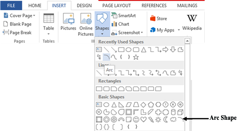
  • On the Insert tab, click on Shapes and select Arc under Basic Shapes
  • Hold down the [Shift] key, click-and-drag to draw an Arc to your desired size
Step 2:           Changing the colour of the object
  • Make sure the object is selected
  • On the Format tab, change the Shape Fill colour to Red and Shape Outline colour to No Outline

Result:
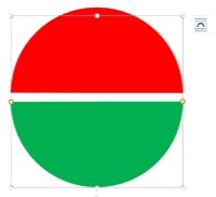
Step 3:           Changing the shape of the object
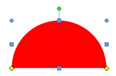
  • Click-and-drag the top Reshape handle (yellow) to the left direction to form a semi-circle


Step 4:           Making a copy of the object
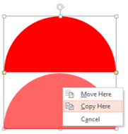
  • Hold down the [Shift] key as you right click-and-drag on the object downwards and release your mouse button
  • From the shortcut menu, select Copy Here
  • Change the Shape Fill colour for the duplicated object to Green
Result:

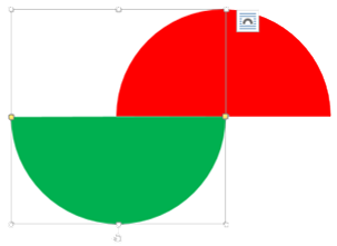
Step 5:           Rotating the object as needed
  • Select the second object you want to rotate upside down
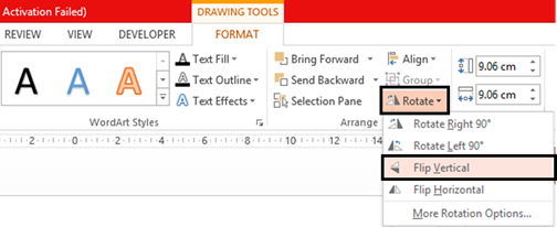
  • On the Format tab, click on Rotate and select Flip Vertically

NB:  The object will be turned upside down (i.e. mirrored)
Note:  You can also hold down the [Shift] key as you click-and-drag on the Free Rotate handle to rotate the object upside down
  • Position the second object to the middle left of the first object as shown below:

Step 6:           Drawing a circle at the middle of the objects
  • On the Insert tab, click on Shapes and select Oval under Basic Shapes
  • Hold down the [Shift] key and draw a Circle at the middle of the objects
  • Change the Shape Fill colour to Yellow; Shape Outline colour to White and Weight to 3pt respectively

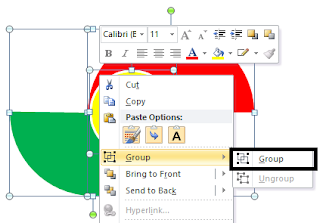
Step 7:           Grouping the objects as needed
  • On the Home tab, click on Select drop-down arrow and click on Select Objects
  • Click-and-drag over the objects to select all
  • Right-click on the selected objects, point to Group and select Group

Note:  You can also hold down the [Shift] key as you click on each object to select for grouping

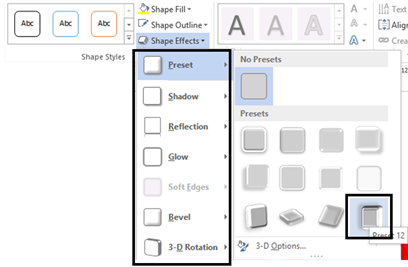
Step 8:           Applying 3D effects to the object
  • With the object still selected, click on Format tab, click on Shape Effects, point to Preset and select Preset 12
  • Change the Bevel to Cool Slant and 3D Rotation to Perspective Contrasting Left respectively

Final Result:

  • Save the document as TV3 logo in a private folder or on your Flash drive

Self-Challenge
  • Use Arc and Wave illustrated shapes respectively to design a Pepsi logo.

  • Apply 3D effects of your choice to the object
  • Save the document as Pepsi Logo in a private folder or on your Flash drive

Note:  

I will continually be adding other practical tutorials ranging from Windows Paint to Adobe Photoshop every week

Source: BB Series

BB's Popular Posts